The Matrix
Continuing from part 1 the matrix form used needs to be described.
If you need a quick "tutorial" in systems of linear equations, take a look at this text I wrote.
First, the vector of the unknowns - x . The vector is:
\large \mathbf{x} = [ G_1 , G_2 , G_3 , \cdots , G_N ]
where GN is the conductance of the respective resistor. We do not know the values of the individual conductances (we know the values of some of the conductances, the reference resistors, but for the purposes of the calculation we do not know them).
The coefficients matrix and the right hand side vector go hand in hand. In the matrix form of equations each equation can be transcribed into one row of the A matrix and one number in the b vector. So for every measured situation we will generate the following equation:
\large (U_1 - U_C) G_1 + (U_2 - U_C)G_2 + ... + (U_N - U_C)G_N = 0
The particular number in b will be 0. As for the row in the matrix A the values will be 0 for the resistors that are not involved in that particular resistive divider and (UN - UC), where UN is the voltage on the node that is connected by RN to the center node and UC is the node on the center voltage
So, let's use the following 8 node system as an example:
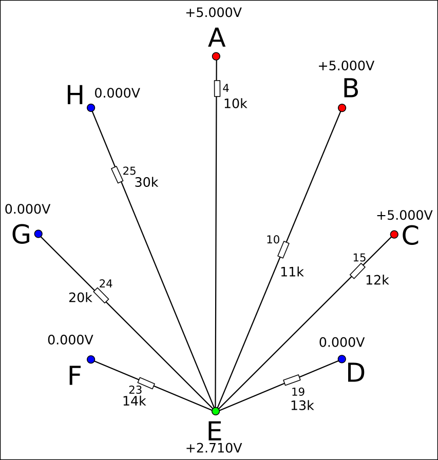
The resistors are numbered. We will apply a situation to it - the measurement system will connect some of the nodes to the low excitation voltage, some to the high excitation voltage and set one to be a high impedance node. Red markers on the image will represent nodes connected to a high excitation voltage, blue nodes represent the ones connected to the low excitation voltage and the green one is the high impedance one that will be the center node for the voltage divider.
| Node | State |
|---|---|
| A | High +5V |
| B | High +5V |
| C | High +5V |
| D | Low GND (0V) |
| E | High impedance (HiZ analog input) |
| F | Low GND (0V) |
| G | Low GND (0V) |
| H | Low GND (0V) |
Connecting the nodes turns the whole setup into a voltage divider. As was discussed previously, we can safely ignore all of the resistors that do not connect directly to the divider center node (E). So, let's connect the nodes. The voltages on the individual nodes will be something like this:
We can safely omit the resistors that are not connected to the center node (E) for clarity. The resistance values are not needed for the actual calculation or matrix formation. Node voltages have been measured as follows:
| Node | Voltage to ground [V] | Resistor connecting to center node (E) |
|---|---|---|
| A | 5.000 | 10k |
| B | 5.000 | 11k |
| C | 5.000 | 12k |
| D | 0.000 | 13k |
| E | 2.710 | N/A |
| F | 0.000 | 14k |
| G | 0.000 | 20k |
| H | 0.000 | 30k |
Only resistors 4, 10, 15, 19, 23, 24, and 25 are involved in the divider. So let's formulate the equation:
(note: Since the equations are getting very long and I'm having trouble fitting them into latex in any way that makes them look good, some will not be written in latex. Appologies to the font nazis.)
0G1 + 0G2 + 0G3 + (UA-UE)G4 + 0G5 + 0G6 + 0G7 + 0G8 + 0G9 + (UB-UE)G10 + 0G11 +
0G12 + 0G13 + 0G14 + (UC-UE)G15 + 0G16 + 0G17 + 0G18 +
(UF-UE)G23 + (UG-UE)G24 + (UH-UE)G25 + 0G26 + 0G27 + 0G28 = 0
Nasty, isn't it? Note however that most of the conductances have a zero coefficient, as such we can remove them.
(U_A - U_E)G_{4} + (U_B - U_E)G_{10} + (U_C - U_E)G_{15} + (U_D - U_E)G_{19} +
(U_F - U_E)G_{23} + (U_G - U_E)G_{24} + (U_H - U_E)G_{25} = 0
Adding the specific numbers we get:
(5-2.710)G_{4} + (5-2.710)G_{10} + (5-2.710)G_{15} + (0-2.710)G_{19} +
(0-2.710)G_{23} + (0-2.710)G_{24} + (0-2.710)G_{25} = 0
Which equals:
2.29 G_{4} + 2.29 G_{10} + 2.29 G_{15} -2.71 G_{19} -2.71 G_{23} -2.71 G_{24} -2.71 G_{25} = 0
So this particular row of the equation will be:
x = (G1 G2 G3 G4   G5 G6 G7 G8 G9 G10  G11 G12 G13 G14 G15  G16 G17 G18 G19   G20 G21 G22 G23   G24   G25   G26 G27 G28)
A = [0  0  0  2.29 0  0  0  0  0  2.29 0   0   0   0   2.29 0   0   0   -2.71 0   0   0   -2.71 -2.71 -2.71 0   0   0]
and that row in b will be 0.
This was the process for creating one single line of the final matrix. For a complete measurement this will have to be repeated many times over for different situations, with the high impedance node set to different nodes.
The absolutely minimal number of different measured situations would be equal to the number of unknown resistances. However, the more situations are measured, the better. With a low number of measured situations the error of the system can be very large (hundreds of percent even, depending on the noise and various other factors, will be discussed in another part). With more measured situations, the error drops down.
The number of possible combinations of node settings (situations) can be pretty large. Assuming that every combination with a single floating node is used, for an 8 node system, assuming two power rails, this comes to 8*128=1024 possible situations. However, not all of them are actually useful - a combination where all of the powered nodes are connected to GND will not yield anything useful, since the resulting divider will be completely connected to one excitation voltage, giving no clues as to the ratios of the resistors. Also, using all of the combinations would cause the measurement to be very long and memory hungry - it's possible, but not needed. So a limited subset is sufficient for an actual measurement. Of the 1024 combinations possible for an 8 node system, I have chosen to use 248 situations, but other numbers of combinations would work as well.
The visual representation of the situations for an 8 node system follows:
This is a representation of 248 situations in the 8 node system. Each "row" represents one situation, each "column" represents one of the nodes. Blue represents a node that is set into a high impedance state, green represents a node tied to GND (low excitation) and red represents a node tied to VCC (high excitation). If you with to see situation visualizations and their source files, please download the following file.
So that's the main part of the matrix - the measurement values. At the moment there are no absolutes present in the matrix. So the reference part of the matrix needs to be added. This is a very different format of an equation. This just assigns a known value to the known resistors. So, assuming that we know the resistances (conductances) of resistors R1, R14 and R28, we will have three reference equations. These are in the following format:
1 G_{N} = g_{N}
where g_{N} is the actual conductance, placed into the right hand side. For the example case, where we know the resistances of R1 (330050 Ohms = 3.029844E-06 S), R14 (329280 Ohms = 3.036929E-06 S) and R28 (329580 Ohms = 3.034165E-06 S) the equations would look as follows:
1 G_{1}=3.029844*10^{-6}
1 G_{14}=3.036929*10^{-6}
1 G_{28}=3.034165*10^{-6}
These lines can be duplicated to further "enforce" this "rule" for the solver. These are the precisely measured values of three 330k resistors that are used as reference resistors on one particular measurement board I made.
That's that as far as the linear equations are concerned. All that is needed is to solve them.
The actual solving is done using a linear equations solver. In the software I made I use Math.NET, but any should do. Basically, the solver searches for a set of values (the x vector) that satisfies all of the equations that are structured into the \textbf{Ax=b} . If no exact solution is possible (which is certainly the case for equations generated this measurement), it searches for a set of values for x that is closest to fitting the equations. The output of a solver is a filled x vector that is the closest solution to the generated measurement.
Now the x vector is filled with the conductivities of the individual resistors. To get the resistances, the reciprocal value of the vector is needed. Once that is gained, we are done - we have the resistances of the individual measured elements. And all it took was a lot of GPIO twiddling and a load of math. Enjoy!
Example
An example matrix, from an actual measurement done using an ATMega32 (the actual implementation of the measurement will be talked about in another part of this series), including an Octave script can be downloaded here:
Unzip the directory somewhere and run the LoadAndCalculate.m script. This is the result of a measurement of a board with resistors of a fixed value, three of which were known reference resistors (R1, R14 and R28).
#Demonstration to load an example resistor net
#matrix and calculate the resistances
#Load the A matrix and the b vector
A = csvread('A.csv');
b = csvread('b.csv');

#Do the actual calculation
x = A\b;

Conductances = x;
#convert the conductances into resistances
Resistances = 1./Conductances;

Resistances' %Display the resistance vector
How the actual calculation works is outside of the scope of this text. See my other post for a very simplified explanations that's probably full of errors, or better yet - read a different text from someone who is actually a mathematician.
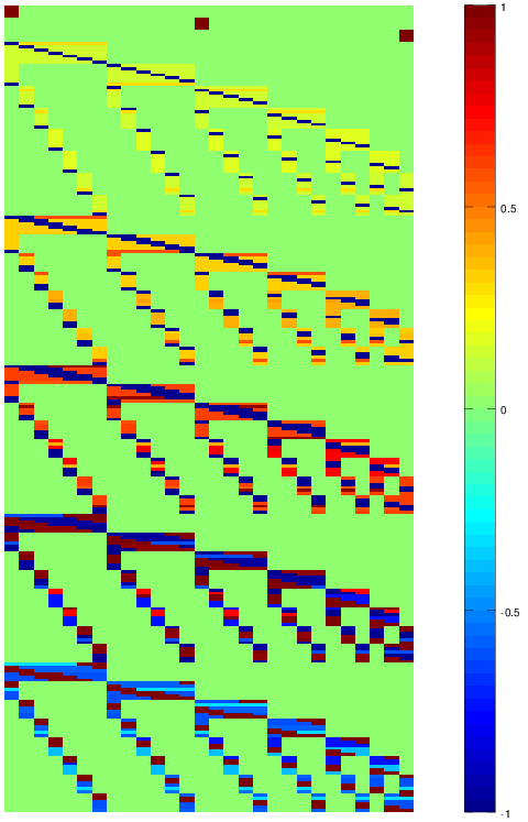
The visual representation of such a matrix (done by PlotMatrix.m ) can be seen here:
This is a visualization of a single matrix. The upper few lines are the reference part of the matrix, the rest are the actual measurement. All lines of the b vector are zero, aside from the ones in the reference part of the matrix. This particular matrix is 260 rows long and 28 columns wide. Of the 260 rows, 12 are the reference part of the equations. The particular pattern that the matrix looks like is explained by how the situation generator generates the situations.
Executing this script should yield the resistances of the individual resistors. In this case they were 25 thermistors, with a 680k resistance at 25 °C, as well as three 330k reference resistors.
Conclusion - method
So, that's that! With this method you can do a measurement of a large quantity of resistors, using a minimal amount of cabling. This is not exactly useful for most areas, and it won't be replacing Kelvin resistance measurements any time soon, but there are niche areas where this method can be actually useful.
Space constrained applications are one area - imagine you have to measure a lot of temperature sensors on the length of a very thin, long rod - any other method would require more cabling or intelligent (capable of connecting to a data bus) sensors. This method just requires say, 16 signals running through the inside of the shaft and you can measure over a hundred thermistors along the length of the shaft. MEMS systems could also benefit from this. Or just a sensor array.
Another interesting usage of this might be using it to measure small quantities of resistors using a lot of known resistors - this actually yielded some interesting results - thanks to the insane amount of oversampling, this can actually provide a resolution well beyond that of the ADC (I'm still working on this area, but the preliminary results are interesting).
The advantages of this measurement are obvious - you can measure a lot of resistors using just the bare minimum amount of cabling or pins of your device, without needing any intelligence in the sensors themselves.
The downside - it's a memory and computation hungry method, it's not exactly fast and there are unforeseeable sources of errors. As such it needs some processor capable of doing the number crunching.
The technique bears some similarity to electrical impedance tomography, but is at its core different for being used on discrete parts (resistors) rather then volumes, uses DC excitation and uses reference resistors to enable the measurement of the exact resistance values. Also, it can be used with a single, cheap microcontroller.
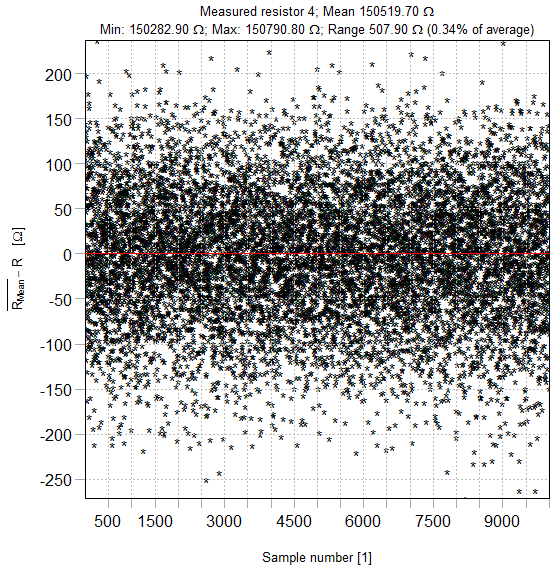
In the next part of this text I will show you a device I built that actually implements this measurement, the software that goes with it and the results. As a teaser I am including the results of an actual measurement of a 150kΩ resistor, which was measured with 27 other resistors 😉 Stay tuned!
And if you liked this text, donations are always welcome!
If you need any help implementing this method for your particular thingamajig, contact me!


4 Responses to New method for measuring lots of resistors using very few wires - part 2 - Theory