Introduction
This article describes a new method of measuring a lot of resistors using a low amount of wires and a lot of math. The resistors can be any kind of resistors, thermistors or other resistive sensors. It can be used in niche applications where space or cabling amount is a problem, where using lots of intelligent sensors that connect onto a bus would be impractical and similar applications.
The method allows you to connect up to N_R = \frac{N_W (N_W-1)}{2} resistors, using just NW wires. For 8 wires that's up to 28 resistors. For 16 wires it's 120 resistors.
I have implemented this method both in theory, simulation and as an actual device. The results are very positive and show that the method can be implemented on cheap of the shelf microcontrollers without much effort (I used an ATMega32).
Update/clarification: The ATMega32 is only the acquisition system - the actual number crunching is done on a PC where a .Net application I wrote does the actual calculation. The ATMega32 is the physical bit.
Origin of the idea
A few years ago, I got the idea that it could be fun to solve one of those nasty EE puzzles/exercises where you start out with a horrible mess of wires and resistors and you are supposed to calculate the resistance between two nodes. At the time I was also fascinated by charlieplexing - an awesome technique that either allows you to control many polarized LEDs (or similar) that are connected in a specific way, or read a lot of buttons. There are some trade-offs you must be willing to accept, but aside from those it's awesome.
I played with it a bit and that got me thinking further, if you could do some kind of more analog measurements via charlieplexing. A bit of pondering later, I found out that you couldn't, it became a horrible mess. But you could use the same kind of setup as is used for charlieplexing (every node is connected by one connection to every other node - a complete graph from a topological view point, or leave out a few connections if they are not needed) to do something different.
After dusting off Norton and Thevenin, relearning systems of linear equations, and poking and prodding other areas of math, I finally arrived at how you can convert the horrible mess of equations that describe a complete graph of resistors into a nice overdetermined system of of linear equations.
The method
Let's assume you have a system of resistors that is connected up in the following way:
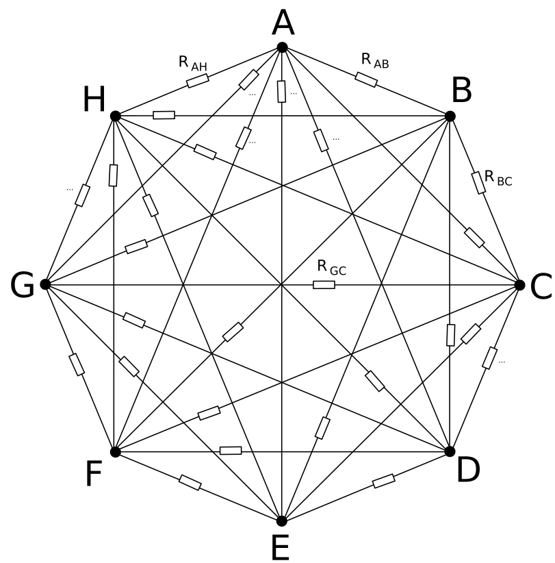
An 8 node version of the measured system
The circles at the corners of the graph are nodes. These connect into the measurement system that will be discussed later. The rectangles are resistors. They may be known (reference resistors) or unknown (measured resistors) - these can be resistive sensing elements, or fixed resistors. Between any two nodes a maximum of one resistor connection can be present. Assuming N nodes this gives us a maximum of N_R = \frac{N (N-1)}{2} resistors. Some of these must be reference resistors, the rest can be unknown.
Every node can be connected to either one of two or more power nets (such as GND and +VCC) - in that case it is referred to as powered node (they will be shown as either red (+VCC) or blue (GND) filled dots), or can be turned into a high impedance state, in which case it is referred to as a high impedance node (and will be shown as a green filled circle). The voltage on every node must be measured (or assumed - if limited accuracy is OK it can be assumed that once a node is connected to GND or +VCC, it is at a constant value - this assumption ignores the GPIO output driver resistance) by an ADC. The nodes can be driven and measured by standard GPIOs, provided the microcontroller can measure the voltage on the pin at the same time it is driving it - Atmels' AVRs can do this, I'm not sure about other MCU families.
A set of node settings (such as A=VCC, B=GND, C=HiZ, D=VCC...) is called a situation.
The role of the measurement system is to connect the individual nodes to their respective power rail depending on the chosen situation, measure the voltage on them (both when they are in a high impedance state and when they are powered) via an ADC, store the values and report them back to a higher system that will compile them into a matrix and crunch the numbers. Fortunately, a simple microcontroller can do all of these things, though a more complex implementation should yield much better results.
Measuring a resistance between any two points is pointless - all of the resistors contribute to the measured value in a horrible series - parallel combination.
However, when a voltage is applied between any two or more nodes, and all of the node voltages are known (by measuring them), there is a way to limit the scope of what needs to be included in the model. Namely it needs to be viewed as a simple resistive divider with a center viewed from one of the high impedance nodes.
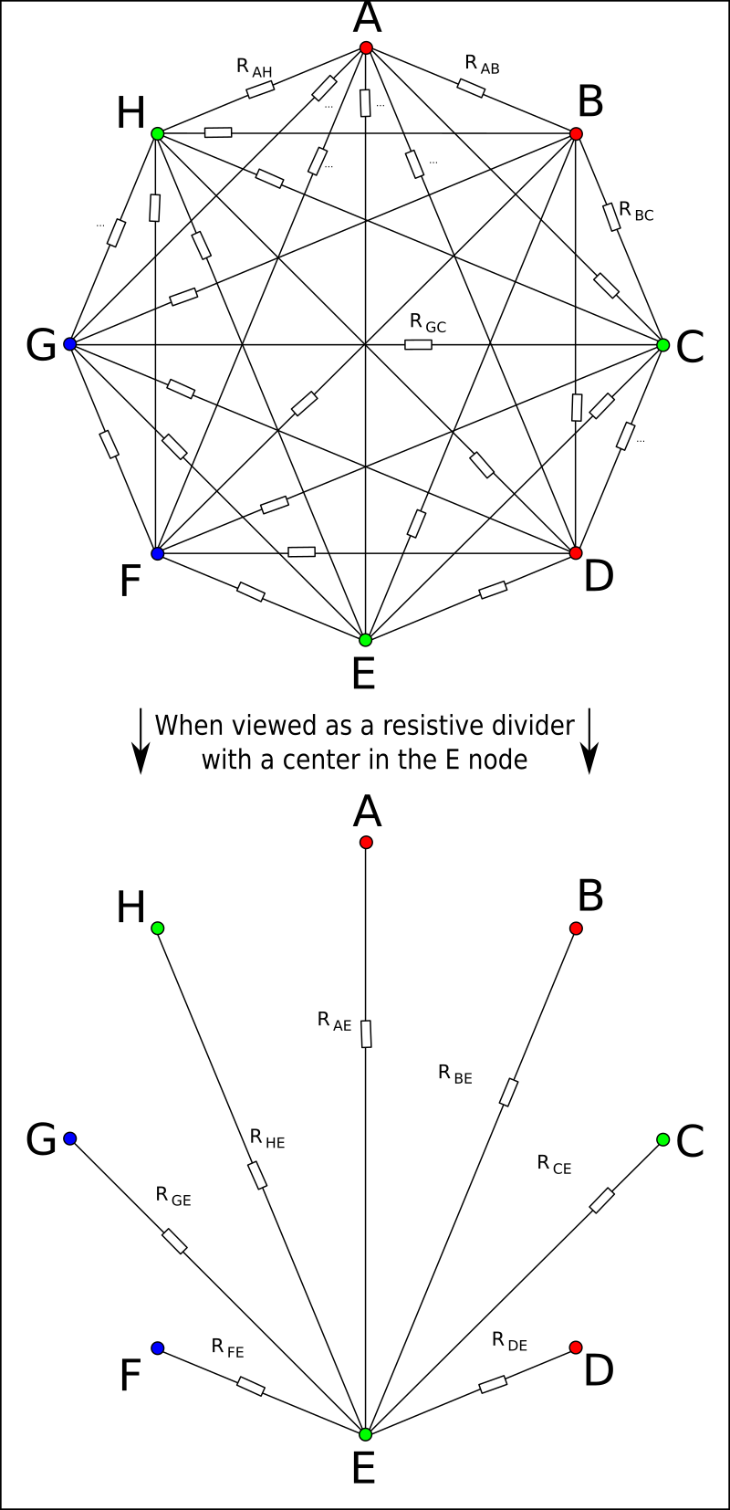
Measured system converted into a resistive divider
When viewed as a resistive divider we can ignore all of the resistors that do not connect the center node (in this case the node E). This greatly simplifies the schematic, from a horrible mess to a simple resistive divider - which in turn will simplify the equations of this particular setup.
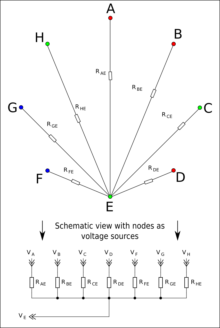
Schematic view of converter block of the resistive network
The general equations for a resistive divider with a single center node and known voltages on its inputs is simple:
\LARGE U_C = ( \sum \frac{U_N}{R_N})(\frac{1}{\sum \frac{1}{R_N}})
Where UN are the individual node voltages, RN is the resistance of the resistor connected between the center node and the other node. The sum needs to be done for all nodes that are connected to the center node by a resistance.
Since we do not know the individual RN values, but we know the voltages we can try to put it into the form of a linear equation. Rewriting the resistances as their reciprocal value - GN (their conductances) gives us the following equation:
\large U_C = ( \sum U_N G_N ) ( \frac{1}{\sum G_N} )
After a bit of fiddling about we can rearrange the whole thing into a nicer form:
\large 0 = U_C \sum G_N - \sum U_N G_N
Another rearrangement gets us this:
\large 0 = \sum U_N G_N - U_C \sum G_N
Note that in this equation we have nothing but multiplying unknowns by knowns - no division, no squares and everything is on one side of the equation. Evaluating this equation yields this:
\large (U_1 - U_C) G_1 + (U_2 - U_C)G_2 + ... + (U_N - U_C)G_N = 0
So, there we have it - note that the unknowns (the conductivities of the measured resistors) are being multiplied by a constant. The resistors (conductivities) that were not involved in the specific situation will not come into this equation and as such they have a coefficient of 0.
It might not seem like much, and for one measured combination of node settings (one situation) such an equation is not particularly useful. However, we can build an overdetermined system of linear equations out of this in a matrix form:
\LARGE \textbf{Ax=b}
where A is the matrix form of the known coefficients, x is the vector of the unknowns (the conductivities) and b is the vector of the constants. If you are not familiar with systems of linear equations, take a look at a little text I wrote on the topic.
So, what will the A matrix look like and how does it come together? What's b? What's x? Can hamburgers see the future?

Pingback: New Method for Measuring Lots of Resistors Using Very Few Wires | Hackaday
Pingback: Calculate every resistor in a network from the outside | Tahium